Kuzushiji is a form of classical Japanese writing that is analogous to older forms of cursive in English. It's no longer used as a common form of writing, but is present in religious calligraphy and classical literature. In this post, I'm going to walk you through the process I used in training a classification model in order to implement a simple OCR (Optical Character Recognition) program for Kuzushiji.

A common classification task involving images involves classifying numbers in the MNIST dataset. Each image in the dataset is in grayscale, ranging from black (0) to white (255). These images are also scaled down to 28 by 28 pixels, resulting 784 features: one for each pixel. However, an important thing to note is that there's only 10 classes, 0 through 9. There are 60k training images and 10k testing images, resulting in around 6k images to train and 1k to test. This is sufficient to provide models with around 99% accuracy using an SVM.

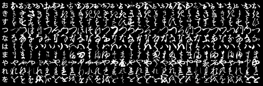
The KMNIST Dataset provided by the Center for Open Data in the Humanities offers a "drop-in replacement" for the MNIST Dataset, with three different datasets: Kuzushiji-KMNIST, Kuzushiji-49, and Kuzushiji-Kanji. In my exploration, I will focus on Kuzushiji-49. Similarly the MNIST, the images are 28 by 28, in 0-255 grayscale. However, Kuzushiji-49 has almost 5 times the number of classes coming in at 49 distinct classes. This means there are significantly more images, up to nearly 271k from 70k. Here is an example of what these images look like:

We'll be focusing on using an SVM in this task, because we'll be comparing against the 99% accuracy that SVMs can achieve on traditional MNIST. Take a look at the repository here for the notebooks I made.

To begin, we should reshape our images from 28 by 28 to one array of length 784.

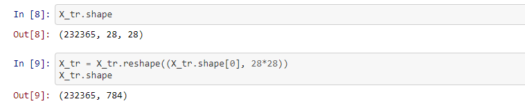
This lets us format our data in traditional format used in SVM models. Secondly, it's useful to look at how these images look at that resolution, because we may find that we need to do some pre-processing such as binarizing.

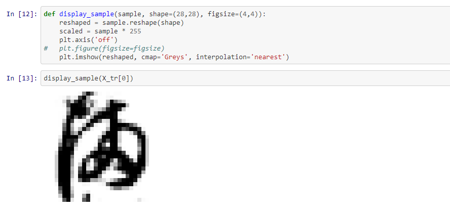
We can see that the strokes of the character have a bit of "fuzz" around the edges, which is expected. One approach that may help is binarizing our images at a certain threshold, to turn grayscale into black/white. An example from the Naive Bayes Notebook is here:

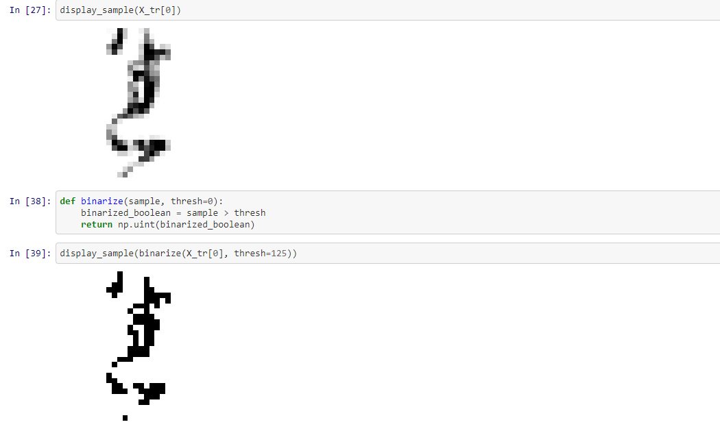
Unfortunately, it looks like binarizing didn't really help with the SVM model, so we're moving forward without that.

Scikit-learn provides a standard scalar preprocessing tool so we can remove the mean and scale to variance in order for our data not to be skewed by very high values which only represent pure black (255). We can also utilize the scikit-learn pipeline tool in order to very easily fit and predict using standard scalar and our model:

Next, we can train, save our model, and predict:

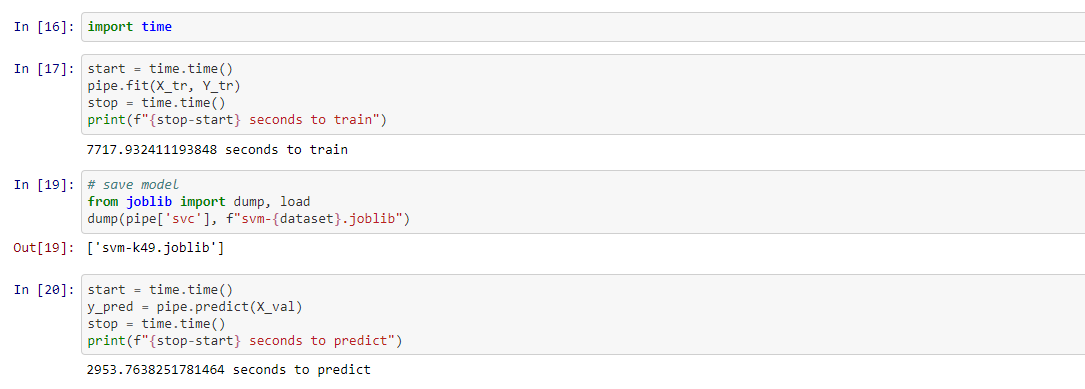
We can see that saving the model was essential: taking over two hours to train means that we can't really afford to re-train each time we want to make predictions. Our model suffers from this long training time due to SVM's limitations with high dimensionality, a problem which may be helped by binarizing or other pre-processing techniques. Notably, our model (svm-k49) comes in at around 850MB, incredibly large and due to the numpy arrays not being compressed.

However, our patience comes with a reward:

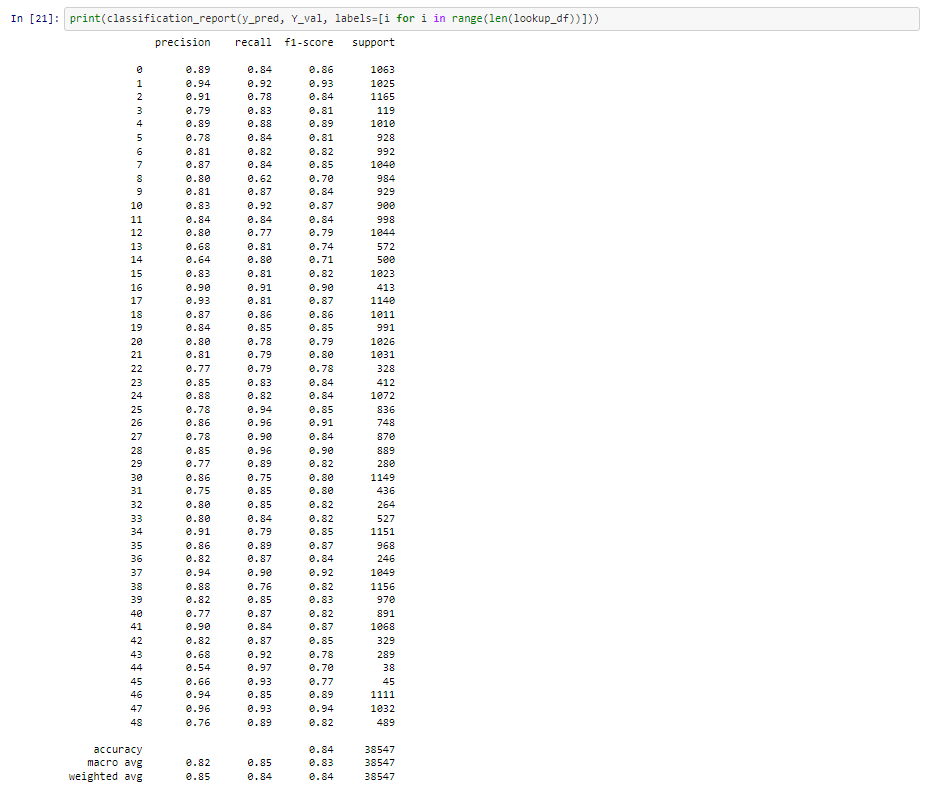
Our model has an f1 score of 84%, which is very good for a model classifying between 49 classes and with minimal pre-processing. There's a big problem though: training and predicting using an SVM took nearly three hours! (2 hours and 57 minutes) This is pretty impractical and uncompetitive. Using a neural network, we can achieve 85% accuracy with less than 5 minutes of training time.

We begin the same up to pre-processing, where we need to reshape our Y targets to one-hot encoded matrices.

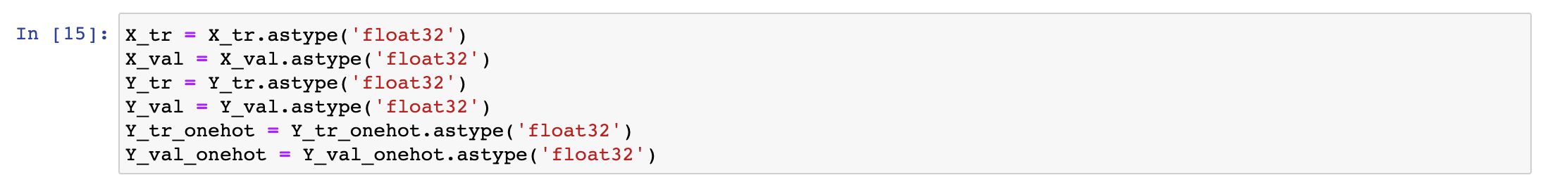
Keras has a utility which makes this simple, so it's just two lines to do it for both our training and testing partitions. Second, we need to convert all of our datatypes to float32 for our Tensorflow model. Tensorflow expects floats, so we need to ensure that we're not giving uints or ints.

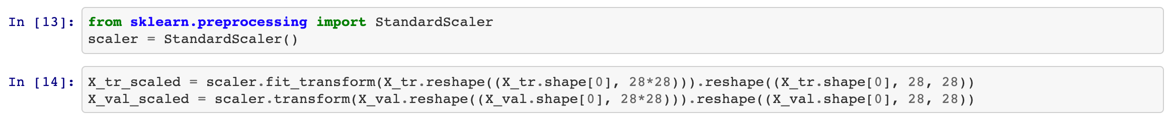
In the last step for preprocessing, we need to standardize our features. Scikit-learn's StandardScaler only allows for numpy arrays of 2 dimensions or lower and our k49 dataset is 3 dimensional. We need to both fit transform and reshape. We can do this in two lines, one for train and one for test. We only fit and transform for our training, since we don't want to refit for our test set.

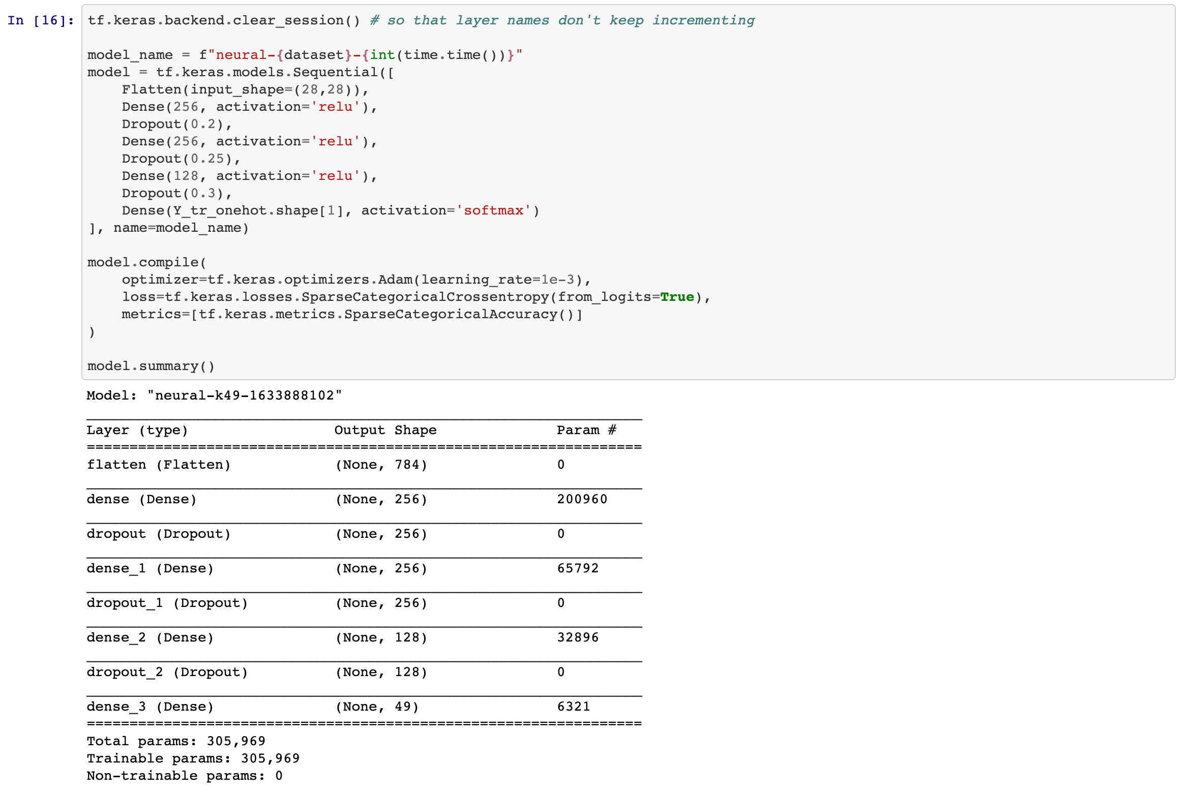
Finally, we can be begin to create our model. We have an input layer, and output layer, and 3 layers in between. All layers have the relu activation function. Our first layer has 256 neurons with a dropout of 0.2, the second is the same but with a dropout of 0.25. Our last layer begins to trim things down to 128 neurons and a dropout of 0.3. We use these dropouts to randomly "turn off" neurons so that a handful of neurons aren't singlehandedly determining our resulting predictions. Our output layer has a simple softmax activation and 49 neurons, one for each class.

Additionally, we're compiling our model using the Adam optimizer with a fairly reasonable learning rate. Our loss and metric accuracy functions are SparseCategoricalCrossentropy, since we're using one-hot encoded targets.

Next, we just need to call the .fit function on the model with our data:

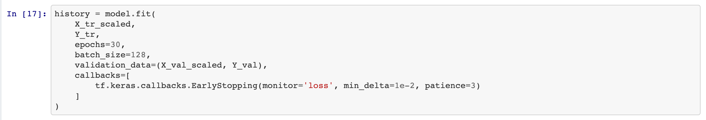
We use our scaled training data for this task. We're also going to tell the fit function to train over 30 epochs, with a batch size of 128. This batch size helps ensure we're getting enough coverage of our 49 classes in each batch. We're also going to include validation data so we can see how the model progresses in each epoch. This data isn't used to influence training, so it's okay to use it. Implementing an early stopping callback for if the loss doesn't make 1e-2 difference since the last epoch would be helpful, but in practice I did reach 30 epochs since each epoch made enough progress on the loss function to avoid early stopping.

Our model evaluates at 85.4% accuracy, which is better than our SVM, and only took about 5 minutes of training and about a second to predict. Lots of improvement!

In fact, we can see in this heat map that we have a nice diagonal line for our 49 classes:

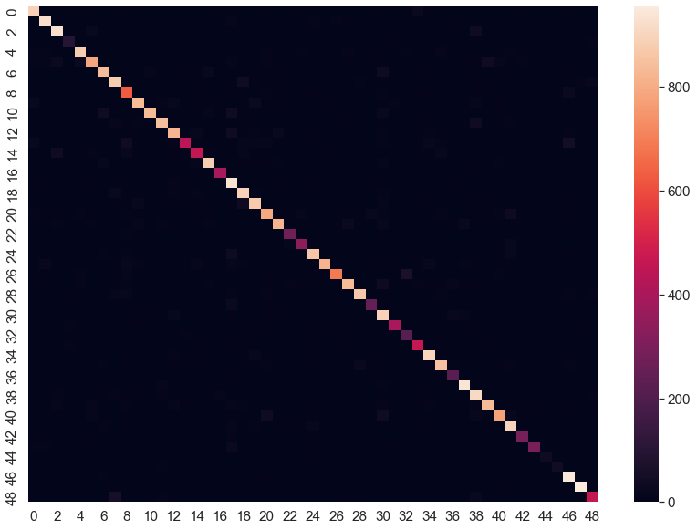
In some cases we have poor performance, such as for our 4th, 43rd, and 44th classes. However, overall we have very good performance when we keep in mind this is over 49 classes.

What's the story here? I argue that while MNIST is used as a baseline to introduce computer vision tasks to students, there is a significant difficulty gap between the well defined 0-9 to what we encounter in the "real-world." Therefore, using a dataset such as KMNIST to parallel MNIST, then moving to k49, we can better understand how dataset size and noise relates to F1 and model complexity.

For more reading, I recommend reading the paper which created the KMNIST dataset.